Data Preparation and Standardization
This page will be used to comment and understand the steps, advances and doubts about the process of data preparation and standardization of the SISTRAT C1 (Convenio 1) which can be translated to Agreement on Collaboration, Technical Assistance and Transfer of Resources to General Population (“Convenio de Colaboración Técnica y de Transferencia de Recursos para Programa de Población General”). Must note that it does not include Adolescent criminal offenders (C2).
To see the TOP or Profile of Treatment Results (“Perfil de Resultados de Tratamiento”) data preparation, go to this webpage.
Building dataset
Define working directories that contain different text files that will be merged, correspondent to the years of the C1 Sistrat.
dir_c1 <-paste0(gsub("/SUD_CL","",path),"/Encriptado c1/Personas tratadas c1/")
dir_top <-paste0(gsub("/SUD_CL","",path),"/encriptados TOP/")
#In my case,
#dir_c1 <-toString(paste0("G:/Mi unidad/Alvacast/SISTRAT 2019 (github)","/Encriptado c1/Personas tratadas c1/"))
#dir_top <-toString(paste0("G:/Mi unidad/Alvacast/SISTRAT 2019 (github)","/encriptados TOP/"))
Define files in the Directory folder, as long as they have the excel extension and they do not start with ~ (represent a working temporary file in excel)
SISTRAT_c1<-list.files(path=toString(dir_c1), all.files=T, pattern="^[2].*\\s*txt$")SISTRAT_c1 is composed by the following files: * 2010tab-Resultado-20191113 (1).txt * 2011tab -Resultado-20191113.txt * 2012tab-Resultado-20191113.txt * 2013tab-Resultado-20191113.txt * 2014tab-Resultado-20191113.txt * 2015tab-Resultado-20191113.txt * 2016tab-Resultado-20191113.txt * 2017tab-Resultado-20191113.txt * 2018tab-Resultado-20191113.txt * 2019_EneOcttab-Resultado-20191113.txt
Function to read tab delimited text files, with UTF-8 encoding and, based on the first 7 letters of its name, assign them an object name.
read_excel_mult <- function(dir, filename) {
  assign(paste0(substr(filename, 1, 7)),read.delim(paste0(dir, filename),
        na.strings="null", header = T, fileEncoding="UTF-8"),envir = .GlobalEnv)
  }
Import datasets
To import the datasets, we apply the previous function to every dataset
for (x in SISTRAT_c1) {
  read_excel_mult(as.character(dir_c1), x)
}
Normalize datasets
Normalize datasets by defining a common name for hash key’s (“HASH_KEY”) and assign them a standardized name.
tab_10_18_mod <- function(x,y) {  get(x) %>% dplyr::rename("HASH_KEY" = !!names(.[91])) %>%
    as.data.frame() %>%
    assign(paste0(y, as.character(x)),.,envir = .GlobalEnv)
}
for (i in paste0(c(2010:2018),"tab")) {tab_10_18_mod(i,y="c1_")}

`2019_En` %>% dplyr::rename("HASH_KEY" = !!names(.[92])) %>%
  as.data.frame() %>%
  assign(paste0("c1_", "2019tab"),.,envir = .GlobalEnv)
Append the datasets
Once column names are normalized, bind every year’s datasets by their rows.
CONS_C1=rbindlist(mget(paste0("c1_",c(2010:2019),"tab")), idcol="TABLE", fill=T)
CONS_C1 <- CONS_C1 %>% dplyr::mutate(row=1:nrow(CONS_C1)) %>% dplyr::select(row,everything())
Define and format variable names
Redefine variable names, create a column named ano_bd with the year. Also, reorder the variables to get the identifiers in the first columns.
Rename Variables
CONS_C1 %>%
  dplyr::rename(id=`Codigo.Identificación`) %>%
  dplyr::rename(fech_ing=`Fecha.Ingreso.a.Tratamiento`) %>%
  dplyr::rename(fech_egres=`Fecha.Egreso.de.Tratamiento`) %>%
  dplyr::rename(dias_trat=`Dias.en.Tratamiento`) %>%
  dplyr::rename(eva_consumo=`Evaluación.al.Egreso.Respecto.al.Patrón.de.consumo`) %>%
  dplyr::rename(eva_fam=`Evaluación.al.Egreso.Respecto.a.Situación.Familiar`) %>%
  dplyr::rename(eva_sm=`Evaluación.al.Egreso.Respecto.Salud.Mental`) %>%
  dplyr::rename(eva_fisica=`Evaluación.al.Egreso.Respecto.Salud.Física`) %>%
  dplyr::rename(eva_transgnorma=`Evaluación.al.Egreso.Respecto.Trasgresión.a.la.Norma.Social`) %>%
  dplyr::rename(eva_relinterp=`Evaluación.al.Egreso.Respecto.Relaciones.Interpersonales`) %>%
  dplyr::rename(eva_ocupacion=`Evaluación.al.Egreso.Respecto.a.Situación.Ocupacional`) %>%
  dplyr::rename(evaluacindelprocesoteraputico=`Evaluación.del.Proceso.Terapéutico`) %>%
  dplyr::rename(nmesesentratamiento=`N.Meses.en.Tratamiento`) %>%
  dplyr::rename(motivodeegreso=`Motivo.de.Egreso`) %>%
  dplyr::rename(tipo_centro=`Tipo.Centro`) %>%
  dplyr::mutate(ano_bd=as.numeric(substr(TABLE,4,7))) %>%
  select(row, TABLE, HASH_KEY,ano_bd, everything()) %>%
  dplyr::arrange(id) %>%
  assign("CONS_C1_df",.,envir = .GlobalEnv)
Relevant variables are converted into factors.
CONS_C1_df %>%
  dplyr::mutate(motivodeegreso=as.factor(motivodeegreso)) %>%
  dplyr::mutate(evaluacindelprocesoteraputico=as.factor(evaluacindelprocesoteraputico)) %>%
  dplyr::mutate(eva_consumo=as.factor(eva_consumo)) %>%
  dplyr::mutate(eva_fam=as.factor(eva_fam)) %>%
  dplyr::mutate(eva_relinterp=as.factor(eva_relinterp)) %>%
  dplyr::mutate(eva_ocupacion=as.factor(eva_ocupacion)) %>%
  dplyr::mutate(eva_sm=as.factor(eva_sm)) %>%
  dplyr::mutate(eva_fisica=as.factor(eva_fisica)) %>%
  dplyr::mutate(eva_transgnorma=as.factor(eva_transgnorma)) %>%
  dplyr::mutate(sexo=as.factor(Sexo)) %>%
  dplyr::mutate(embarazo=as.factor(`X.Se.trata.de.una.mujer.embarazada.`)) %>%
  dplyr::mutate(tipo_de_plan=as.factor(`Tipo.de.Plan`)) %>%
  dplyr::mutate(tipo_de_programa=as.factor(`Tipo.de.Programa`)) %>%
#ACTUALIZATION: JANUARY 2020
  dplyr::mutate(`tipo_centro`=as.factor(`tipo_centro`)) %>%
  dplyr::mutate(`Servicio.de.Salud`=as.factor(`Servicio.de.Salud`)) %>%
  dplyr::mutate(SENDA=as.factor(SENDA)) %>%
  dplyr::mutate(Origen.de.Ingreso=as.factor(Origen.de.Ingreso)) %>%
  dplyr::mutate(País.Nacimiento=as.factor(País.Nacimiento)) %>%
  dplyr::mutate(Nacionalidad=as.factor(Nacionalidad)) %>%
  dplyr::mutate(Etnia=as.factor(Etnia)) %>%
  dplyr::mutate(Estado.Conyugal=as.factor(Estado.Conyugal)) %>%
  dplyr::mutate(Sustancia.de.Inicio=as.factor(Sustancia.de.Inicio)) %>%
  dplyr::mutate(X.Se.trata.de.una.mujer.embarazada.=as.factor(X.Se.trata.de.una.mujer.embarazada.)) %>%
  dplyr::mutate(Escolaridad..último.año.cursado.=as.factor(Escolaridad..último.año.cursado.)) %>%
  dplyr::mutate(Condicion.Ocupacional=as.factor(Condicion.Ocupacional)) %>%
  dplyr::mutate(Categoría.Ocupacional=as.factor(Categoría.Ocupacional)) %>%
  dplyr::mutate(Rubro.Trabaja=as.factor(Rubro.Trabaja)) %>%
  dplyr::mutate(Con.Quién.Vive=as.factor(Con.Quién.Vive)) %>%
  dplyr::mutate(Tipo.de.vivienda=as.factor(Tipo.de.vivienda)) %>%
  dplyr::mutate(Tenencia.de.la.vivienda=as.factor(Tenencia.de.la.vivienda)) %>%
  dplyr::mutate(Sustancia.Principal=as.factor(Sustancia.Principal)) %>%
  dplyr::mutate(Otras.Sustancias.nº1=as.factor(Otras.Sustancias.nº1)) %>%
  dplyr::mutate(Otras.Sustancias.nº2=as.factor(Otras.Sustancias.nº2)) %>%
  dplyr::mutate(Otras.Sustancias.nº3=as.factor(Otras.Sustancias.nº3)) %>%
  dplyr::mutate(Frecuencia.de.Consumo..Sustancia.Principal.=as.factor(Frecuencia.de.Consumo..Sustancia.Principal.)) %>%
  dplyr::mutate(Vía.Administración..Sustancia.Principal.=as.factor(Vía.Administración..Sustancia.Principal.)) %>%
  dplyr::mutate(Diagnóstico.Trs..Consumo.Sustancia=as.factor(Diagnóstico.Trs..Consumo.Sustancia)) %>%
  dplyr::mutate(Diagnóstico.Trs..Psiquiátrico.DSM.IV=as.factor(Diagnóstico.Trs..Psiquiátrico.DSM.IV)) %>%
  dplyr::mutate(Diagnóstico.Trs..Psiquiátrico.SUB.DSM.IV=as.factor(Diagnóstico.Trs..Psiquiátrico.SUB.DSM.IV)) %>%
  dplyr::mutate(X2.Diagnóstico.Trs..Psiquiátrico.DSM.IV=as.factor(X2.Diagnóstico.Trs..Psiquiátrico.DSM.IV)) %>%
  dplyr::mutate(X2.Diagnóstico.Trs..Psiquiátrico.SUB.DSM.IV=as.factor(X2.Diagnóstico.Trs..Psiquiátrico.SUB.DSM.IV)) %>%
  dplyr::mutate(X3.Diagnóstico.Trs..Psiquiátrico.DSM.IV=as.factor(X3.Diagnóstico.Trs..Psiquiátrico.DSM.IV)) %>%
  dplyr::mutate(X3.Diagnóstico.Trs..Psiquiátrico.SUB.DSM.IV=as.factor(X3.Diagnóstico.Trs..Psiquiátrico.SUB.DSM.IV)) %>%
  dplyr::mutate(Diagnóstico.Trs..Psiquiátrico.CIE.10=as.factor(Diagnóstico.Trs..Psiquiátrico.CIE.10)) %>%
  dplyr::mutate(Diagnóstico.Trs..Psiquiátrico.SUB.CIE.10=as.factor(Diagnóstico.Trs..Psiquiátrico.SUB.CIE.10)) %>%
  dplyr::mutate(X2.Diagnóstico.Trs..Psiquiátrico.CIE.10=as.factor(X2.Diagnóstico.Trs..Psiquiátrico.CIE.10)) %>%
  dplyr::mutate(X2.Diagnóstico.Trs..Psiquiátrico.SUB.CIE.10=as.factor(X2.Diagnóstico.Trs..Psiquiátrico.SUB.CIE.10)) %>%
  dplyr::mutate(X3.Diagnóstico.Trs..Psiquiátrico.CIE.10=as.factor(X3.Diagnóstico.Trs..Psiquiátrico.CIE.10)) %>%
  dplyr::mutate(X3.Diagnóstico.Trs..Psiquiátrico.SUB.CIE.10=as.factor(X3.Diagnóstico.Trs..Psiquiátrico.SUB.CIE.10)) %>%
  dplyr::mutate(Diagnóstico.Trs..Físico=as.factor(Diagnóstico.Trs..Físico)) %>%
  dplyr::mutate(Otros.Problemas.de.Atención.de.Salud.Mental=as.factor(Otros.Problemas.de.Atención.de.Salud.Mental)) %>%
  dplyr::mutate(Compromiso.Biopsicosocial=as.factor(Compromiso.Biopsicosocial)) %>%
  dplyr::mutate(DIAGNOSTICO.GLOBAL.DE.NECESIDADES.DE.INTEGRACION.SOCIAL=as.factor(DIAGNOSTICO.GLOBAL.DE.NECESIDADES.DE.INTEGRACION.SOCIAL)) %>%
  dplyr::mutate(DIAGNOSTICO.DE.NECESIDADES.DE.INTEGRACIóN.SOCIAL.EN.CAPITAL.HUMANO=as.factor(DIAGNOSTICO.DE.NECESIDADES.DE.INTEGRACIóN.SOCIAL.EN.CAPITAL.HUMANO)) %>%
  dplyr::mutate(DIAGNOSTICO.DE.NECESIDADES.DE.INTEGRACIóN.SOCIAL.EN.CAPITAL.FISICO=as.factor(DIAGNOSTICO.DE.NECESIDADES.DE.INTEGRACIóN.SOCIAL.EN.CAPITAL.FISICO)) %>%
  dplyr::mutate(DIAGNOSTICO.DE.NECESIDADES.DE.INTEGRACIóN.SOCIAL.EN.CAPITAL.SOCIAL=as.factor(DIAGNOSTICO.DE.NECESIDADES.DE.INTEGRACIóN.SOCIAL.EN.CAPITAL.SOCIAL)) %>%
  dplyr::mutate(Usuario.de.Tribunales..Tratamiento.Drogas=as.factor(Usuario.de.Tribunales..Tratamiento.Drogas)) %>%
  dplyr::mutate(Consentimiento.Informado=as.factor(Consentimiento.Informado)) %>%
  dplyr::mutate(motivodeegreso=as.factor(motivodeegreso)) %>%
  dplyr::mutate(Tipo.Centro.Derivación=as.factor(Tipo.Centro.Derivación)) %>%
  dplyr::mutate(evaluacindelprocesoteraputico=as.factor(evaluacindelprocesoteraputico)) %>%
  dplyr::mutate(eva_consumo=as.factor(eva_consumo)) %>%
  dplyr::mutate(eva_fam=as.factor(eva_fam)) %>%
  dplyr::mutate(eva_relinterp=as.factor(eva_relinterp)) %>%
  dplyr::mutate(eva_ocupacion=as.factor(eva_ocupacion)) %>%
  dplyr::mutate(eva_sm=as.factor(eva_sm)) %>%
  dplyr::mutate(eva_fisica=as.factor(eva_fisica)) %>%
  dplyr::mutate(eva_transgnorma=as.factor(eva_transgnorma)) %>%
  dplyr::mutate(Diagnóstico.Trastorno.Psiquiátrico.CIE.10.al.Egreso=as.factor(Diagnóstico.Trastorno.Psiquiátrico.CIE.10.al.Egreso)) %>%
  dplyr::mutate(DIAGNOSTICO.GLOBAL.DE.NECESIDADES.DE.INTEGRACION.SOCIAL.1=as.factor(DIAGNOSTICO.GLOBAL.DE.NECESIDADES.DE.INTEGRACION.SOCIAL.1)) %>%
  dplyr::mutate(DIAGNOSTICO.DE.NECESIDADES.DE.INTEGRACIóN.SOCIAL.EN.CAPITAL.HUMANO.1=as.factor(DIAGNOSTICO.DE.NECESIDADES.DE.INTEGRACIóN.SOCIAL.EN.CAPITAL.HUMANO.1)) %>%
  dplyr::mutate(DIAGNOSTICO.DE.NECESIDADES.DE.INTEGRACIóN.SOCIAL.EN.CAPITAL.FISICO.1=as.factor(DIAGNOSTICO.DE.NECESIDADES.DE.INTEGRACIóN.SOCIAL.EN.CAPITAL.FISICO.1)) %>%
  dplyr::mutate(DIAGNOSTICO.DE.NECESIDADES.DE.INTEGRACIóN.SOCIAL.EN.CAPITAL.SOCIAL.1=as.factor(DIAGNOSTICO.DE.NECESIDADES.DE.INTEGRACIóN.SOCIAL.EN.CAPITAL.SOCIAL.1)) %>%
  dplyr::mutate(Motivo.de.egreso.Alta.Administrativa=as.factor(Motivo.de.egreso.Alta.Administrativa)) %>%
  dplyr::mutate(Ha.estado.embarazada.egreso.=as.factor(Ha.estado.embarazada.egreso.)) %>%
  dplyr::mutate(identidad.de.genero=as.factor(identidad.de.genero)) %>%
  dplyr::mutate(discapacidad=as.factor(discapacidad)) %>%
  dplyr::mutate(Opción.discapacidad=as.factor(Opción.discapacidad)) %>%
  dplyr::mutate(sexo=as.factor(sexo)) %>%
  dplyr::mutate(embarazo=as.factor(embarazo)) %>%
  dplyr::mutate(tipo_de_plan=as.factor(tipo_de_plan)) %>%
  dplyr::mutate(tipo_de_programa=as.factor(tipo_de_programa)) %>%
  assign("CONS_C1_df",.,envir = .GlobalEnv)
Standardize Dates
Dates of admission and discharge
Most of the dates were not formatted equally. When standardized, some cases failed to transform dates, specifically in dates of discharge, which contained 87 cases, while only one case was problematic in admission dates.
CONS_C1_df %>%
  dplyr::mutate(fech_ing= ifelse(row=="14504", "10/01/2011",
                          ifelse(row=="88379", "09/07/2015", #ACTUALIZACION 2020-01-17: change of date of admission
                          ifelse(row=="79428", "09/07/2015", #ACTUALIZACION 2020-01-17: change of date of admission
                                        fech_ing))))  %>%
  dplyr::mutate(fech_ing= lubridate::parse_date_time(fech_ing, c("%d/%m/%Y"),exact=T)) %>% #un caso falla en ser transformado
  dplyr::mutate(fech_egres_sin_fmt= fech_egres) %>% #me quedo con esta variable por si acaso
  dplyr::mutate(fech_egres= ifelse(row=="36308", "02/04/2013",
                            ifelse(row=="14083", "03/05/2011",
                            ifelse(row=="6349", "01/07/2010",
                            ifelse(row=="42741", "02/08/2013",
                            ifelse(row=="8608","01/02/2011",
                            ifelse(row=="11709","01/02/2011",
                            ifelse(row=="40486","03/07/2013",
                            ifelse(row=="42521","09/07/2013",
                            ifelse(row=="5757", "04/10/2010", #cambiado
                            ifelse(row=="39507", "02/07/2013",
                            ifelse(row=="3195", "04/10/2010",
                            ifelse(row=="37845", "01/07/2013",
                            ifelse(row=="40180", "07/08/2013",
                            ifelse(row=="28008", "27/11/2012",
                            ifelse(row=="35971", "01/03/2013",
                            ifelse(row=="5172", "03/05/2011",
                            ifelse(row=="10415", "03/05/2011",
                            ifelse(row=="16385", "30/08/2011",
                            ifelse(row=="39932", "02/08/2013",
                            ifelse(row=="16983", "06/09/2011",
                            ifelse(row=="88379", "11/04/2016", #ACTUALIZATION 2020-01-17: change of date of discharge
                            ifelse(row=="79428", "11/04/2016", #ACTUALIZATION 2020-01-17: change of date of discharge
                            ifelse(row=="37004", "02/08/2013",fech_egres)))))))))))))))))))))))) %>%
  dplyr::mutate(fech_egres= lubridate::parse_date_time(stringr::str_trim(fech_egres),
                                                       orders = c("%d/%m/%Y", "%d/%m/%y","%d%m%Y"),exact=T)) %>%
  dplyr::arrange(desc(ano_bd)) %>%
  assign("CONS_C1_df",.,envir = .GlobalEnv) #87 failed to parse, bajé a 37, y 30 después de quitar espacios
For discharge dates, many cases had different formats. Those had to be transformed once the first formats were traduced (e.g. 30-12-2019 is interpreted first in “%d/%m/%Y” format. If it is not traduced, it interprets in “DD/MM/YY” format (or “%d/%m/%y”). We can see in Table 1 in non-formatted date of discharge (fech_egres_sin_fmt) how it was traduced into an plausible discharge date (fech_egres). One criterion is that in many cases, the second and or third 0 would possibly correspond to a month character. On the contrary, “7082013” or “9072013” would be “2013-8-70” and “2013-7-90”, respectively.
| Case | HASH | ID | Date of Admission | Date of Discharge | Date of Discharge (No Format) | Days in Treatment |
|---|---|---|---|---|---|---|
| 36,308 | b6373dccc2b0b5ffba42db746b17c692 | CAPE1**051992 | 2013-01-29 | 2013-04-02 | 2013/04/02 | NA |
| 42,741 | 090f64b945afce17900e82eccb8f8da6 | COMO2**091988 | 2013-07-02 | 2013-08-02 | 2082013 | NA |
| 40,486 | 4fc0a1cff37ad152767eb323ed3b43c0 | ELPO2**111980 | 2013-05-02 | 2013-07-03 | 307203 | NA |
| 42,521 | c668aa3153ea4a1a4435c45557feb80b | HUDO1**091969 | 2013-06-28 | 2013-07-09 | 9072013 | NA |
| 39,507 | 2f477adf8b5c282660fa16180eb5096d | LIDO2**031992 | 2013-04-29 | 2013-07-02 | 2072013 | NA |
| 37,845 | fd919f36ada0b9423cf3acdead577150 | MAZA1**111968 | 2013-03-18 | 2013-07-01 | 1072013 | NA |
| 40,180 | c8a0c6ccce12e9d3fbc74c06d6a06664 | MIMA2**111973 | 2013-05-29 | 2013-08-07 | 7082013 | NA |
| 35,971 | 132aa32661fbedca4ecdd1e2018c58e3 | PARA1**021977 | 2013-01-02 | 2013-03-01 | 01-03-2013 | NA |
| 39,932 | c87466931290f44c2c6a89bd127d31e5 | RELA2**011969 | 2013-05-22 | 2013-08-02 | 2082013 | NA |
| 37,004 | ad7eb82186ec39a61ad29aed61522c2a | SO-A2**061980 | 2013-02-08 | 2013-08-02 | 2082013 | NA |
| 28,008 | 3d50c479484a18e510d6be8f8a35a1ed | OMHU1**041990 | 2012-06-25 | 2012-11-27 | 27-11-2012 | NA |
| 14,083 | 68930653a30b13a6f6f7853d6683dff3 | CLFI1**031973 | 2011-02-10 | 2011-05-03 | 30520011 | NA |
| 14,504 | a7a1fcb4a638a7b194063d95e34320a9 | CLVE2**111966 | 2011-01-10 | 2011-08-30 | 30/08/2011 | 232 |
| 11,709 | 52eeb63fbce34e95c7687dd6007efce8 | DASA2**031986 | 2008-08-08 | 2011-02-01 | 01-02-2011 | NA |
| 10,415 | 4aa3462c09ad1a7cc1e6d249f620d715 | PATR1**061986 | 2010-04-26 | 2011-05-03 | 3052011 | NA |
| 16,385 | 1454ce9c37a56516ce054a3513361a66 | RAPA1**051983 | 2011-04-18 | 2011-08-30 | 30/08/20011 | NA |
| 16,983 | 5ebc5439f9db863ff8744778280360db | SERI1**011960 | 2011-05-13 | 2011-09-06 | 06-09-2011 | NA |
| 6,349 | 9a8fef6d37e8010c477c25db3e5e8455 | CLGO1**101984 | 2010-06-17 | 2010-07-01 | 01707/2010 | NA |
| 8,608 | 52eeb63fbce34e95c7687dd6007efce8 | DASA2**031986 | 2008-08-08 | 2011-02-01 | 01-02-2011 | NA |
| 5,757 | 4485da22c54dbef2c45c61a92b5f7cac | JAGO1**121972 | 2010-05-03 | 2010-10-04 | 4102010 | NA |
| 3,195 | 07a0a0c984ae3d9dfcd30b55fcb6beb2 | LUME1**091957 | 2009-10-07 | 2010-10-04 | 4102010 | NA |
| 5,172 | 4aa3462c09ad1a7cc1e6d249f620d715 | PATR1**061986 | 2010-04-26 | 2011-05-03 | 3052011 | NA |
As we can see in Table 2, some non-formatted dates of discharge (fech_egres_sin_fmt), had insufficient information to traduce into valid dates.
| Year | case | DischargeDate | DischargeDate-NoFmt |
|---|---|---|---|
| 2,011 | 12,006 | NA | 5 |
| 2,011 | 12,005 | NA | 5 |
| 2,011 | 12,227 | NA | 25 |
| 2,010 | 8,239 | NA | 15 |
| 2,010 | 9,043 | NA | 5 |
| 2,010 | 2,603 | NA | 20/0/2010 |
| 2,010 | 9,042 | NA | 5 |
| 2,010 | 194 | NA | 15 |
| 2,010 | 9,353 | NA | 25 |
UPDATE: 2019-12-11, had to format this date because it was badly labelled. CONS_C1_df[CONS_C1_df$row=="5757","fech_egres"] <- parse_date_time(str_trim("04/10/2010"), orders = c("%d/%m/%Y"),exact=T). UPDATE: 2020-01-17. Thanks to SENDA’s experts, they provided us with information about a case with missing values in dates of treatment. This date had to be formatted because it was badly labeled. CONS_C1_df[CONS_C1_df$row=="88379","fech_ing"] <- parse_date_time(str_trim("09/07/2015"), orders = c("%d/%m/%Y"),exact=T). UPDATE: 2020-01-17, this date had to be formatted because it was badly labeled. CONS_C1_df[CONS_C1_df$row=="79428","fech_ing"] <- parse_date_time(str_trim("09/07/2015"), orders = c("%d/%m/%Y"),exact=T). UPDATE: 2020-01-17, this date had to be formatted because it was badly labeled. CONS_C1_df[CONS_C1_df$row=="88379","fech_egres"] <- parse_date_time(str_trim("11/04/2016"), orders = c("%d/%m/%Y"),exact=T). UPDATE: 2020-01-17, this date had to be formatted because it was badly labeled. CONS_C1_df[CONS_C1_df$row=="79428","fech_egres"] <- parse_date_time(str_trim("11/04/2016"), orders = c("%d/%m/%Y"),exact=T). Still, there are 9752 cases with NULL dates of discharge.
Data Cleaning Steps provided by SENDA’s professional
These rules were provided by SENDA’s professionals, in order to select adequate data for the analysis.
1. Exclude non-SENDA treatments
In the first place, we should discard treatments not provided by SENDA. NULL values correspond to a single HASH key (“72c54d822de128e52f10511f3eb2d19f”, in datasets from 2010 and 2011) that did not have a plan and program.
| SENDA | Frequency | % |
|---|---|---|
| No | 7,762 | 4.8% |
| Si | 155,382 | 95.2% |
| NA | 2 | 0% |
| No= Admission under another agreement | ||
| Si= Admission under SENDA agreement |
As we can see in Table 3, around 4.8% of cases had a treatment that could not be part of SENDA’s agreements. The case that did not take part under SENDA categories was admitted to a SENDA agreement in 2009/12/10 and in 2009/12/14. Attending to what was informed by SENDAs professional in January 2020, many programs that was pointed as not part of SENDA may actually be part of SENDA. That is why we keep these programs anyways, despite what was originally stated.
2. Explore the type of plan
It is necessary to explore if there is any case that may have a treatment under a probation/parole (“libertad vigilada”) plan. It is necessary to consider the 3 null values in type of plans, equivalent to 2 HASHs, dropping the case with a plan in Probation/Parole.
## `summarise()` regrouping output by 'SENDA' (override with `.groups` argument)| Type of Plan | No SENDA(n) | No SENDA(%) | Yes SENDA(n) | Yes SENDA(%) | NA (n) | NA (%) |
|---|---|---|---|---|---|---|
| CALLE | 5 | 0% | 10 | 0% | NA | NA |
| M-PAB | 6 | 0% | 109 | 0% | NA | NA |
| M-PAI | 137 | 2% | 10533 | 7% | NA | NA |
| M-PAI2 | NA | NA | 16 | 0% | NA | NA |
| M-PR | 251 | 3% | 7588 | 5% | NA | NA |
| M-PR2 | NA | NA | 10 | 0% | NA | NA |
| Otro | 1778 | 23% | 90 | 0% | NA | NA |
| PAI LV | NA | NA | 1 | 0% | NA | NA |
| PG-PAB | 2236 | 29% | 54075 | 35% | NA | NA |
| PG-PAI | 2233 | 29% | 66300 | 43% | NA | NA |
| PG-PR | 1116 | 14% | 16599 | 11% | NA | NA |
| PG PAI 2 | NA | NA | 50 | 0% | NA | NA |
| NA | NA | NA | 1 | 0% | 2 | 100% |
| PR= Residential Program | ||||||
| PAB= Basic Outpatient Program | ||||||
| PAI= Intensive Outpatient Treatment | ||||||
| PAI LV= Probation/Parole | ||||||
| PAI= Intensive Outpatient Treatment |
Table 4 shows that there is only 1 case in the probation/parole plan.
3. Changes in programs
Change fixed residential, flexible residential and residential programs into a general population residential program (PG PR). Additionally, flexible residential program cannot be under a probation/parole program.
Must note that there are some plans that have a number 2 but they do not contain more than 0% of the total of the datasets. Also there are some plans related to the Treatment of People Living on the Streets Program (Programa de Tratamiento de Personas en Situación de Calle). We should change plans ‘Otro’ and ‘Calle’ into ‘General Population’. Plans with number 2 should be grouped with their respective plan, leaving only M-PAI, M-PR, PG-PAB, PG-PAI, and PG-PR. For the moment, we are not sure what is the fixed and flexible residential programs.
| Type of Program | CALLE | M-PAB | M-PAI | M-PAI2 | M-PR | M-PR2 | Otro | PAI LV | PG-PAB | PG-PAI | PG-PR | PG PAI 2 | NA |
|---|---|---|---|---|---|---|---|---|---|---|---|---|---|
| Libertad Vigilada | 0 | 0 | 0 | 0 | 0 | 0 | 0 | 0 | 0 | 2 | 0 | 0 | 0 |
| Otro | 0 | 0 | 3 | 0 | 3 | 0 | 890 | 0 | 32 | 35 | 12 | 2 | 0 |
| Programa Alcohol | 0 | 0 | 0 | 0 | 0 | 0 | 0 | 0 | 0 | 80 | 0 | 0 | 0 |
| Programa Calles | 15 | 0 | 0 | 0 | 0 | 0 | 0 | 0 | 0 | 0 | 0 | 0 | 0 |
| Programa Específico Mujeres | 0 | 115 | 9,741 | 16 | 7,590 | 10 | 7 | 0 | 19 | 48 | 3 | 16 | 0 |
| Programa Población General | 0 | 0 | 926 | 0 | 246 | 0 | 971 | 1 | 56,260 | 68,368 | 17,700 | 32 | 0 |
| NA | 0 | 0 | 0 | 0 | 0 | 0 | 0 | 0 | 0 | 0 | 0 | 0 | 3 |
4. Plans within Alcohol Program
If there is a plan within the alcohol program, the plan must be modified into the general population plan.
Every of the 10, 80 cases in the alcohol program should be in the general population plan.
5. Another Plan
If there is any plan correspondent to Another (“Otro”), it changes into a general population program.
There are 1868 cases with treatments categorized as Another (“Otro”) plan.
6. Plan & Programs by Sex
Women should be in the M-PAI in which they actually are categorized in the general population program.
As can be seen in Table 6, around 58% of women are in the general population programs.Should they be removed or changed?
| Plan | Men (n) | Men (%) | Women (n) | Women (%) |
|---|---|---|---|---|
| CALLE | 12 | 0% | 3 | 0% |
| M-PAB | NA | NA | 115 | 0% |
| M-PAI | 86 | 0% | 10,584 | 23% |
| M-PAI2 | NA | NA | 16 | 0% |
| M-PR | 68 | 0% | 7,771 | 17% |
| M-PR2 | NA | NA | 10 | 0% |
| Otro | 1,305 | 1% | 563 | 1% |
| PAI LV | 1 | 0% | NA | NA |
| PG-PAB | 44,527 | 38% | 11,784 | 26% |
| PG-PAI | 54,142 | 46% | 14,391 | 31% |
| PG-PR | 17,057 | 15% | 658 | 1% |
| PG PAI 2 | 27 | 0% | 23 | 0% |
| NA | 3 | 0% | NA | NA |
| PR= Residential Program | ||||
| PAB= Basic Outpatient Program | ||||
| PAI= Intensive Outpatient Treatment | ||||
| PAI LV= Probation/Parole | ||||
| PAI= Intensive Outpatient Treatment |
There are still a few doubts about these criteria:
Why are there men and women with female gender identity that are in the general population?, (Basic outpatient, intensive outpatient, Residential and Outpatient 2)
Should the 2 men and 12 women in M-PAI but with masculine gender identity be in the general population (PG PAI)?
If there is a woman with masculine gender identity in M-PR, should they not be in the general population (PG_PR)?
7. Plan & Programs by Sex
Only plans “M-PAI”, “M-PR”, “PG-PAB”, “PG-PAI” and “PG-PR” must be preserved. Considering Table 4, what happens with M-PAB (basic outpatient for women), “Calle”, “PG PAI 2”, “M-PAI2”, “M-PR2”, “PAI LV” or another (“Otro”)? (See Table 4)
8. Age of consumption onset
Treat the age of consumption onset as missing data if it is less than 5 years.
Figure 1. Histogram of Age of Consumption Begin
  par(mfrow = c(1,2))
  hist(CONS_C1_df$Edad.Inicio.Consumo, main="Distribution of Age\nof Consumption Begin",
       xlab="Age", ylab="Freq", breaks=30, xlim=c(0,80))
  hist(CONS_C1_df$Edad.Inicio.Consumo, main="Distribution of Age\nof Consumption Begin (zoom)",
       xlab="Age", ylab="Freq", breaks=30, xlim=c(0,10), ylim=c(0,20000))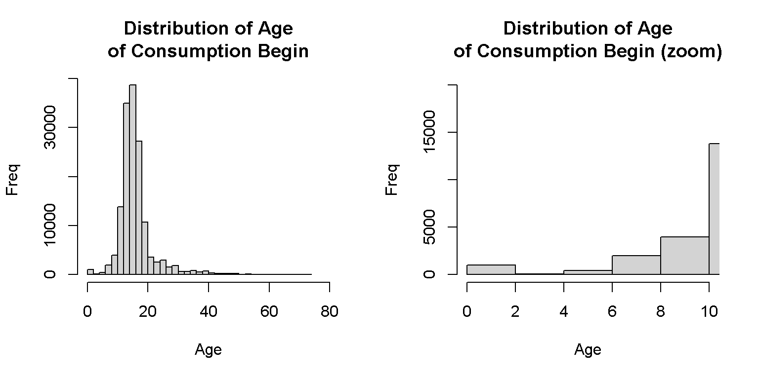
There are around 1117 cases that showed a consumption onset of less than 5 years old. These should be declared as missing data.
9. Delete duplicated cases (same date of admission and ID)
In this case, we included the HASH-KEY as another and more robust criteria to filter duplicate cases.
| Frequencies | Percentage | |
|---|---|---|
| Repeated | 45,526 | 27.9% |
| Unique | 117,620 | 72.1% |
As seen in Table 7, there are more than a quarter of cases that may be replicating across the different datasets. Considering the difficulties involved in determining repeated cases without dropping relevant information due to specific changes, this will be done posteriorly, once dataset is a bit more normalized.
10. Current Age
Consider age as missing age if the case was less than 18 years and greater than 90. UPDATE: This had been reconsidered as a result of a join with SENDA’s professionals, that stated that in specific cases people would have entered treatment when they were not yet adults (<18 years old).
Figure 2. Histogram of Actual Age
    par(mfrow = c(1,3))
    hist(CONS_C1_df$Edad, main="Distrbution of Age",
         xlab="Age", ylab="Freq", breaks=60)
    hist(CONS_C1_df$Edad, main="Distrbution of Age (zoom -)",
         xlab="Age", ylab="Freq", breaks=60, xlim=c(0,20), ylim=c(0,2000))
    hist(CONS_C1_df$Edad, main="Distrbution of Age (zoom +)",
xlab="Age", ylab="Freq", breaks=60, xlim=c(100,120), ylim=c(0,100)) 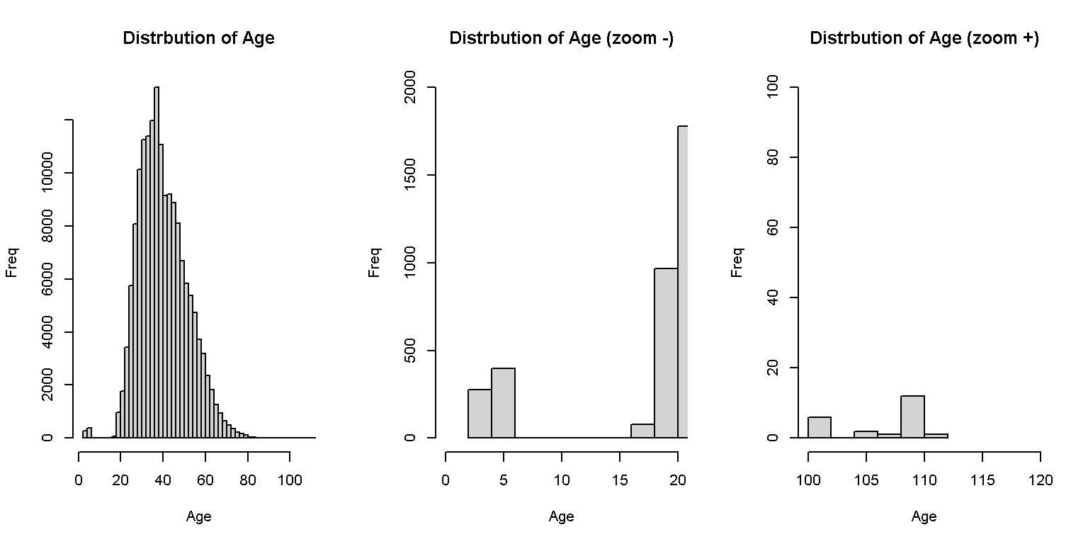
    CONS_C1_df %>%
      dplyr::filter(Edad<18) %>%
      dplyr::summarise(n())

    CONS_C1_df %>%
      dplyr::filter(Edad>90) %>%
      dplyr::summarise(n())
There were 673 cases with less than 18 years, 24 cases with more than 90 years. Considering the complexities involved in the age and what should be done to retrieve it adequately, this will be done posteriorly, once other variables are normalized.
11. Days in Treatment
Consider days in treatment as missing if the case had more than 1095 days. Do the same for months in treatment.
Figure 3. Histogram of Days In Treatment
    par(mfrow = c(1,2))
    hist(CONS_C1_df$dias_trat, main="Distribution of\nDays in Treatment",
         xlab="Days", ylab="Freq",xlim=c(-100,4100), breaks=60)
    hist(CONS_C1_df$dias_trat, main="Distribution of\nDays in Treatment (zoom +)",
xlab="Days", ylab="Freq", breaks=60, xlim=c(1000,4100), ylim=c(0,2000)) 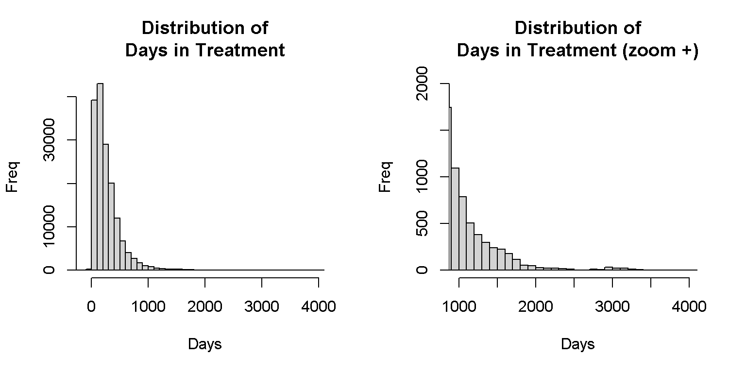
#values out of boundariesAs seen in Figure 3, there are 2320 cases with more than 1095 days in treatment. On the other hand, there are 280 cases with negative or no days of treatment. Due to the complexities involved in the number of treatment days, deletion will be done posteriorly.
12. Pregnancy and Sex
Pregnant men should be considered as missing values. As seen in Table 8, 4 cases of men also reported pregnancy. These cases should be declared as missing.
| Pregnancy | Man (n) | Man (%) | Women (n) | Women (%) |
|---|---|---|---|---|
| No | 9515 | 8% | 43466 | 95% |
| Si | 4 | 0% | 2430 | 5% |
| NA | 107709 | 92% | 22 | 0% |
| Si= Pregnant | ||||
| No= Not Pregnant |
13. Type of plan and Sex
See plans M-PR and M-PAI. Check if there are men. Keep the entries only if they identify as women.
As seen in Table 9, it must be noted that many cases do not answer this question, or perhaps it’s more plausible, this question was not present in previous datasets. This is why we may exclude NA’s (missing values) for the following analysis.
| Gender Identity | Man (n) | Man (%) | Women (n) | Women (%) |
|---|---|---|---|---|
| Femenino | 65 | 0% | 3249 | 7% |
| Masculino | 8012 | 7% | 60 | 0% |
| NA | 109151 | 93% | 42609 | 93% |
| Femenino= Feminine | ||||
| Masculino= Masculine |
In Table 10, it can be seen that there are 2 men with a masculine gender identity that are subscribed to the M-PAI plan. However, what happens with the women with masculine gender identity in the M-PAI plan?
| Plan | Fem.-Men(n) | Fem.-Men(%) | Masc.-Men(n) | Masc.-Men(%) | Fem.-Women(n) | Fem.-Women(%) | Masc.-Women(n) | Masc.-Women(%) |
|---|---|---|---|---|---|---|---|---|
| M-PAI | 2 | 3% | 2 | 0% | 877 | 27% | 12 | 20% |
| M-PAI2 | NA | NA | NA | NA | 16 | 0% | NA | NA |
| M-PR | 2 | 3% | NA | NA | 505 | 16% | 1 | 2% |
| M-PR2 | NA | NA | NA | NA | 10 | 0% | NA | NA |
| Otro | 1 | 2% | 25 | 0% | 15 | 0% | NA | NA |
| PG-PAB | 22 | 34% | 2688 | 34% | 690 | 21% | 19 | 32% |
| PG-PAI | 33 | 51% | 4060 | 51% | 1098 | 34% | 28 | 47% |
| PG-PR | 5 | 8% | 1212 | 15% | 26 | 1% | NA | NA |
| PG PAI 2 | NA | NA | 25 | 0% | 12 | 0% | NA | NA |
| PR= Residential Program | ||||||||
| PAB= Basic Outpatient Program | ||||||||
| PAI= Intensive Outpatient Treatment | ||||||||
| PAI LV= Probation/Parole | ||||||||
| PAI= Intensive Outpatient Treatment |
This can be done by replacing plans of men with masculine identities that are in M- plans, into the General Population. This should be resolved in the following secitons.
14. Days of treatment
Consider days of treatment as missing if there are values of 0 and negative values.
As shown in Figure 3, there are 280 values of 0 or negative values. This must be resolved once treatment days are standardized and overlappings in treatments are corrected.
    CONS_C1_df %>%
    dplyr::filter(dias_trat<1) %>%
      dplyr::select(-id,-TABLE,-14,-16,-17,-26,-27,-28,-29,-35,-36,-37,-88,-93,-94,-96,-101) %>%
      dplyr::select(row, ano_bd, HASH_KEY, hash_rut_completo, id_mod, dias_trat,fech_ing, fech_egres,tipo_de_plan, tipo_de_programa,
                    ID.centro,motivodeegreso, everything()) %>%
      head() %>%
 knitr::kable(.,format = "html", format.args = list(decimal.mark = ".", big.mark = ","),
               caption="Table 11. Cases with lower dates of treatment",
                 align =rep('c', 101))  %>%
  kable_styling(bootstrap_options = c("striped", "hover"),font_size = 8) %>%
scroll_box(width = "100%", height = "350px")| row | ano_bd | HASH_KEY | hash_rut_completo | id_mod | dias_trat | fech_ing | fech_egres | tipo_de_plan | tipo_de_programa | ID.centro | motivodeegreso | Nombre.Centro | tipo_centro | Región.del.Centro | Servicio.de.Salud | Tipo.de.Programa | Tipo.de.Plan | SENDA | Dias.en.SENDA | Edad | Nombre.Usuario | Comuna.Residencia | Origen.de.Ingreso | País.Nacimiento | Nacionalidad | Etnia | Estado.Conyugal | Fecha.Ultimo.Tratamiento | Sustancia.de.Inicio | Edad.Inicio.Consumo | X.Se.trata.de.una.mujer.embarazada. | Escolaridad..último.año.cursado. | Con.Quién.Vive | Tipo.de.vivienda | Tenencia.de.la.vivienda | Sustancia.Principal | Otras.Sustancias.nº1 | Otras.Sustancias.nº2 | Otras.Sustancias.nº3 | Frecuencia.de.Consumo..Sustancia.Principal. | Edad.Inicio..Sustancia.Principal. | Vía.Administración..Sustancia.Principal. | Diagnóstico.Trs..Consumo.Sustancia | Diagnóstico.Trs..Psiquiátrico.DSM.IV | Diagnóstico.Trs..Psiquiátrico.SUB.DSM.IV | X2.Diagnóstico.Trs..Psiquiátrico.DSM.IV | X2.Diagnóstico.Trs..Psiquiátrico.SUB.DSM.IV | X3.Diagnóstico.Trs..Psiquiátrico.DSM.IV | X3.Diagnóstico.Trs..Psiquiátrico.SUB.DSM.IV | Diagnóstico.Trs..Psiquiátrico.CIE.10 | Diagnóstico.Trs..Psiquiátrico.SUB.CIE.10 | X2.Diagnóstico.Trs..Psiquiátrico.CIE.10 | X2.Diagnóstico.Trs..Psiquiátrico.SUB.CIE.10 | X3.Diagnóstico.Trs..Psiquiátrico.CIE.10 | X3.Diagnóstico.Trs..Psiquiátrico.SUB.CIE.10 | Diagnóstico.Trs..Físico | Otros.Problemas.de.Atención.de.Salud.Mental | Compromiso.Biopsicosocial | DIAGNOSTICO.GLOBAL.DE.NECESIDADES.DE.INTEGRACION.SOCIAL | DIAGNOSTICO.DE.NECESIDADES.DE.INTEGRACIóN.SOCIAL.EN.CAPITAL.HUMANO | DIAGNOSTICO.DE.NECESIDADES.DE.INTEGRACIóN.SOCIAL.EN.CAPITAL.FISICO | DIAGNOSTICO.DE.NECESIDADES.DE.INTEGRACIóN.SOCIAL.EN.CAPITAL.SOCIAL | Fecha.Ingreso.a.Convenio.SENDA | Usuario.de.Tribunales..Tratamiento.Drogas | Consentimiento.Informado | Tipo.Centro.Derivación | evaluacindelprocesoteraputico | eva_consumo | eva_fam | eva_relinterp | eva_ocupacion | eva_sm | eva_fisica | eva_transgnorma | Diagnóstico.Trastorno.Psiquiátrico.CIE.10.al.Egreso | DIAGNOSTICO.GLOBAL.DE.NECESIDADES.DE.INTEGRACION.SOCIAL.1 | DIAGNOSTICO.DE.NECESIDADES.DE.INTEGRACIóN.SOCIAL.EN.CAPITAL.HUMANO.1 | DIAGNOSTICO.DE.NECESIDADES.DE.INTEGRACIóN.SOCIAL.EN.CAPITAL.FISICO.1 | DIAGNOSTICO.DE.NECESIDADES.DE.INTEGRACIóN.SOCIAL.EN.CAPITAL.SOCIAL.1 | Motivo.de.egreso.Alta.Administrativa | Consorcio | Ha.estado.embarazada.egreso. | sexo | embarazo | ano_nac |
|---|---|---|---|---|---|---|---|---|---|---|---|---|---|---|---|---|---|---|---|---|---|---|---|---|---|---|---|---|---|---|---|---|---|---|---|---|---|---|---|---|---|---|---|---|---|---|---|---|---|---|---|---|---|---|---|---|---|---|---|---|---|---|---|---|---|---|---|---|---|---|---|---|---|---|---|---|---|---|---|---|---|---|---|---|---|
| 53,692 | 2,014 | 44e3de7dae9efc5f37695d7bef2a19ee | CAGA2**121982 | 0 | 2014-01-28 | 2014-01-28 | M-PR | Programa Específico Mujeres | 159 | Abandono | Comunidad Terapeutica Crem (Hogares Crem) | privado | METROPOLITANA | Metropolitano Oriente | Programa Específico Mujeres | M-PR | Si | 0 | 36 | OCULTO | MACUL | Otro Centro Tratamiento Drogas | Chile | Chile | No pertenece | Soltero | último 6 meses | Alcohol | 13 | No | UNIVERSITARIA INCOMPLETA | Únicamente con hijos y padres o familia de origen | Casa | Allegado | Alcohol | Cocaína | Marihuana | Hongos | 4-6 días - semana | 13 | Oral (bebida o comida) | Dependencia | En estudio | NA | NA | NA | NA | NA | En estudio | NA | NA | NA | NA | NA | Sin trastorno | Abuso Sexual | Severo | NA | NA | NA | NA | 28/01/2014 | No | Si | NA | Logro M?mo | Logro Mínimo | Logro Mínimo | Logro Mínimo | Logro Mínimo | Logro Mínimo | Logro Mínimo | Logro Mínimo | NA | NA | NA | NA | NA | NA | Opazo y Compañia Ltda. | NA | Mujer | No | 1,982 | |
| 53,553 | 2,014 | 86abe004a5c39f635f562c49d2329f7d | JODI2**021993 | 0 | 2014-01-06 | 2014-01-06 | Otro | Programa Específico Mujeres | 219 | Alta Admnistrativa | Comunidad Terapeutica Romeral (Dianova Mujeres Maule) | privado | DEL MAULE | Maule | Programa Específico Mujeres | Otro | Si | 0 | 26 | OCULTO | TALCA | Otros de la Red de Salud General Público | Chile | Chile | No pertenece | Soltero | último 6 meses | Marihuana | 13 | No | BASICA INCOMPLETA | Únicamente con padres o familia de origen | Casa | Allegado | Pasta Base | Marihuana | NA | NA | Todos los días | 15 | Fumada o Pulmonar (aspiración de gases o vapores) | Dependencia | NA | NA | NA | NA | NA | NA | En estudio | NA | NA | NA | NA | NA | ETS | Explotaci?omercial Sexual | Moderado | NA | NA | NA | NA | 06/01/2014 | No | Si | NA | Logro M?mo | Logro Mínimo | Logro Mínimo | Logro Mínimo | Logro Mínimo | Logro Mínimo | Logro Mínimo | Logro Mínimo | NA | NA | NA | NA | NA | NA | ONG. Dianova Chile | NA | Mujer | No | 1,993 | |
| 53,402 | 2,014 | ac3c9557b7a403430b8058e3099fa221 | PAAL1**071976 | 0 | 2014-01-27 | 2014-01-27 | Otro | Programa Población General | 303 | Alta Admnistrativa | CTR Nehuen (Residencial Melipilla) | publico | METROPOLITANA | Metropolitano Occidente | Programa Población General | Otro | Si | 0 | 43 | OCULTO | MELIPILLA | Consulta Espontánea | Chile | Chile | No pertenece | Casado | último 12 meses | Alcohol | 19 | NA | BASICA COMPLETA | Únicamente con la pareja e hijos | Mediagua | Propia | Pasta Base | NA | NA | NA | 2-3 días - semana | 24 | Fumada o Pulmonar (aspiración de gases o vapores) | Dependencia | NA | NA | NA | NA | NA | NA | En estudio | NA | NA | NA | NA | NA | En estudio | Sin otros problemas de salud mental | Severo | NA | NA | NA | NA | 27/01/2014 | No | Si | NA | Logro M?mo | Logro Mínimo | Logro Mínimo | Logro Mínimo | Logro Mínimo | Logro Mínimo | Logro Mínimo | Logro Mínimo | NA | NA | NA | NA | NA | NA | SERVICIO DE SALUD METROPOLITANO OCCIDENTE | NA | Hombre | NA | 1,976 | |
| 36,706 | 2,013 | b24c50c72c85669ea416ec86b3b11681 | ALAC1**031981 | 0 | 2013-02-04 | 2013-02-04 | PG-PAI | Programa Población General | 148 | Abandono | COSAM Quilicura | publico | METROPOLITANA | Metropolitano Norte | Programa Población General | PG-PAI | No | NA | 38 | OCULTO | QUILICURA | Consulta Espontánea | Chile | Chile | No pertenece | Soltero | NA | Marihuana | 17 | NA | MEDIA COMPLETA | Únicamente con pareja | NA | NA | Pasta Base | NA | NA | NA | 4-6 días - semana | 28 | Fumada o Pulmonar (aspiración de gases o vapores) | Dependencia | NA | NA | NA | NA | NA | NA | En estudio | NA | NA | NA | NA | NA | Sin trastorno | Otros | Severo | NA | NA | NA | NA | NA | No | Si | NA | Logro M?mo | Logro Mínimo | Logro Mínimo | Logro Mínimo | Logro Mínimo | Logro Mínimo | Logro Mínimo | Logro Mínimo | NA | NA | NA | NA | NA | NA | SERVICIO DE SALUD METROPOLITANO NORTE | NA | Hombre | NA | 1,981 | |
| 36,713 | 2,013 | c4f4e254f4e5224db6b81d5f0fdddb6e | ALAG1**021994 | 0 | 2013-02-06 | 2013-02-06 | PG-PAI | Programa Población General | NA | Derivación | NA | NA | NA | NA | Programa Población General | PG-PAI | Si | 0 | 25 | OCULTO | SANTIAGO CENTRO | Otros de la Red de Salud General Privado | Chile | Chile | Mapuche | Casado | NA | Alcohol | 0 | NA | BASICA COMPLETA | Solo | Casa | Arrienda | Alcohol | Marihuana | Cocaína | Pasta Base | Todos los días | 12 | Fumada o Pulmonar (aspiración de gases o vapores) | Dependencia | NA | NA | NA | NA | NA | NA | En estudio | NA | NA | NA | NA | NA | Otras Enfermedades o Condiciones de Riesgo Vital | NA | Severo | NA | NA | NA | NA | 06/02/2013 | No | Si | Otro Centro | Logro M?mo | Logro Alto | Logro Alto | Logro Alto | Logro Alto | Logro Alto | Logro Intermedio | Logro Alto | NA | NA | NA | NA | NA | NA | NA | NA | Hombre | NA | 1,994 | |
| 45,004 | 2,013 | ace460ae4527071c9039dc91dfd58092 | ALCA1**121956 | 0 | 2013-10-14 | 2013-10-14 | PG-PAB | Programa Población General | 241 | Alta Admnistrativa | CRS La Florida | publico | METROPOLITANA | Metropolitano Sur Oriente | Programa Población General | PG-PAB | No | NA | 62 | OCULTO | LA FLORIDA | Estab. de APS | Chile | Chile | No pertenece | Casado | NA | Alcohol | 16 | NA | MEDIA INCOMPLETA | Únicamente con la pareja e hijos | Departamento | Propia | Alcohol | Cocaína | NA | NA | 2-3 días - semana | 16 | Oral (bebida o comida) | Consumo Perjudicial | En estudio | NA | NA | NA | NA | NA | En estudio | NA | NA | NA | NA | NA | En estudio | Sin otros problemas de salud mental | Moderado | NA | NA | NA | NA | NA | No | No | NA | Logro M?mo | Logro Mínimo | Logro Mínimo | Logro Mínimo | Logro Mínimo | Logro Mínimo | Logro Mínimo | Logro Mínimo | NA | NA | NA | NA | NA | NA | SERVICIO DE SALUD METROPOLITANO SUR ORIENTE | NA | Hombre | NA | 1,956 |
15. Age of Consumption Onset and Current Age
Consider the age of consumption onset as missing data if it is greater than the current age.
In 780 cases, the age of consumption onset is greater than the current age. This will be corrected once ages are normalized.
CONS_C1_df %>% dplyr::mutate(edad_inicio_cons= ifelse(Edad.Inicio.Consumo>Edad, 1, 0)) %>% dplyr::filter(edad_inicio_cons==1) %>%
  dplyr::select(row, HASH_KEY, ano_bd, id_mod, Edad.Inicio.Consumo,Edad) %>%
  head(50) %>%
 knitr::kable(.,format = "html", format.args = list(decimal.mark = ".", big.mark = ","),
               caption="Table 12. Cases with age of consumption begin greater than the actual age",
                 align =rep('c', 101))  %>%
  kable_styling(bootstrap_options = c("striped", "hover"),font_size = 8) %>%
scroll_box(width = "100%", height = "350px")| row | HASH_KEY | ano_bd | id_mod | Edad.Inicio.Consumo | Edad |
|---|---|---|---|---|---|
| 155,268 | fb74493f56becc488867fe53c5573a08 | 2,019 | ALAL2**012001 | 25 | 18 |
| 161,209 | 2a33829bf3464ee50d4c8c5087a81093 | 2,019 | CORU2**021992 | 32 | 27 |
| 150,494 | 69c9e351e5132a9b487eaeaea44c0c77 | 2,019 | GOMI1**062000 | 25 | 19 |
| 158,818 | d6d3a38f49580254e4a9a876b2209b29 | 2,019 | ISAM1**062001 | 20 | 18 |
| 151,947 | 910ad076dd1e17a321519f65c5feaa99 | 2,019 | JALI1**061979 | 52 | 40 |
| 160,567 | 4935ae99848d64148eb2f1a0230c4ebb | 2,019 | KATE2**072001 | 24 | 18 |
| 159,445 | a0eee7839dc689824f91b86db156f82f | 2,019 | MAES2**072001 | 22 | 18 |
| 153,734 | 7d92e6e8d55a12c1b308c78dbad0f5b9 | 2,019 | MAPE1**031995 | 29 | 24 |
| 148,287 | e586f94b6247f0e208a906f97f2420f2 | 2,019 | NECU1**052000 | 21 | 19 |
| 146,598 | 1d91d6b2b75fe7a4d8e2a8dfebcfa16c | 2,019 | NELA1**121999 | 54 | 19 |
| 159,705 | a6929b6c7987cce64b0ca1b3f3299bea | 2,019 | ROCO2**072001 | 20 | 18 |
| 160,788 | f90dd528fbe2005a3a3cf88e4f873c83 | 2,019 | RUTR2**051997 | 24 | 22 |
| 131,749 | 9018b21f72370bdeca005ab540d7c7be | 2,018 | ALNE1**101999 | 25 | 20 |
| 127,314 | fc87d7f86b4e9f568fb50eccb29f3891 | 2,018 | ANAR1**041999 | 24 | 20 |
| 136,733 | 07402f400b254ee4662b8a831365612b | 2,018 | DIJI1**051992 | 34 | 27 |
| 138,430 | 445bfb8e194056cb920c163d851c3f92 | 2,018 | ELCA1**052000 | 30 | 19 |
| 125,808 | 578ae693be289de023125ddd2777dd1c | 2,018 | GARO1**012015 | 15 | 4 |
| 144,205 | 69c9e351e5132a9b487eaeaea44c0c77 | 2,018 | GOMI1**062000 | 25 | 19 |
| 125,800 | 8d2dfe24c7a24d541a13b4e82b82eede | 2,018 | HEAV1**112014 | 13 | 4 |
| 131,633 | e0a8c5bbde98b9ed30a52230a7a8b0cb | 2,018 | JACE2**061999 | 50 | 20 |
| 142,720 | 0c9be3e89c1a7576227d2204aada9c24 | 2,018 | JUVA1**111993 | 26 | 25 |
| 126,276 | 9b2836d1a04bffaf371d93392573f692 | 2,018 | MAGU2**051996 | 43 | 23 |
| 129,532 | b24908c527faa1b7bd5a267d5dcabd45 | 2,018 | MAHE2**091999 | 62 | 20 |
| 131,012 | eaf995cb33d947ef6b637e0f89907f96 | 2,018 | MIPE1**091999 | 25 | 20 |
| 127,827 | 6fc3007c689e78c3a6af220449514b4e | 2,018 | MYLO2**051986 | 46 | 33 |
| 140,084 | e586f94b6247f0e208a906f97f2420f2 | 2,018 | NECU1**052000 | 21 | 19 |
| 133,368 | 1d91d6b2b75fe7a4d8e2a8dfebcfa16c | 2,018 | NELA1**121999 | 54 | 19 |
| 130,850 | 865d8750fff6ca0711f52527bcd70b96 | 2,018 | PAAV2**101997 | 25 | 22 |
| 129,149 | ac8234f0a33399c702103d076a9a8de5 | 2,018 | REVA2**081999 | 30 | 20 |
| 132,807 | 2174b5058b56e4471af11248a73f215b | 2,018 | ROVE1**121999 | 25 | 19 |
| 125,944 | 711029aaa5f478f2c55223d285eb84fe | 2,018 | SHMA1**082013 | 15 | 6 |
| 127,280 | 45fce40da4dfc892ba5d4154f8d6b5b6 | 2,018 | SOVA2**121998 | 46 | 20 |
| 125,778 | ad16844e62fd0a0db5ddd59ccffccbf6 | 2,018 | SUUB2**102013 | 26 | 6 |
| 127,320 | 5ca64697dd399116abdd351906e52ab1 | 2,018 | YESA1**031999 | 21 | 20 |
| 136,457 | 744991c3ca5e12e87f2a7925d254e5f6 | 2,018 | YOBO2**022000 | 23 | 19 |
| 125,184 | 9018b21f72370bdeca005ab540d7c7be | 2,017 | ALNE1**101999 | 25 | 20 |
| 116,020 | fc87d7f86b4e9f568fb50eccb29f3891 | 2,017 | ANAR1**041999 | 24 | 20 |
| 106,706 | c51ce03a395b620b21a70b0d028a77e6 | 2,017 | ANMA1**031996 | 27 | 23 |
| 120,750 | bde31338de6a454e11a31da13e9aa8ee | 2,017 | BAGA2**041996 | 25 | 23 |
| 106,134 | 68a1abebf175673e62b97b65fde63b50 | 2,017 | BRHE1**092015 | 15 | 4 |
| 119,326 | 4908c125c91bed71becbd7cf1077e5b2 | 2,017 | CALU2**071999 | 24 | 20 |
| 105,458 | 2cdd842e8b1102992ff2c060e7b46178 | 2,017 | CASA1**122014 | 18 | 4 |
| 105,847 | 87afef689812b1ad6f576f0e83e5c963 | 2,017 | DABU1**032015 | 14 | 4 |
| 107,001 | 31d3a088c8730a02c4ef7239a02e511f | 2,017 | DIBU2**041996 | 30 | 23 |
| 105,661 | 0d5782868d35d58892a0f938813f7608 | 2,017 | EDHO1**052015 | 17 | 4 |
| 106,644 | 2817347e37b21d9ff166af0685b417ff | 2,017 | ENSA1**031996 | 25 | 23 |
| 108,082 | d9e020a08875ef763ce0c3e06cbf1b9d | 2,017 | ERVA1**081995 | 25 | 24 |
| 124,962 | 99246ebba3341f26ce047e32d9c3742b | 2,017 | FEJA1**121999 | 36 | 19 |
| 105,599 | e89eb1528cbb255f7a94ade170a93768 | 2,017 | FRJA1**042015 | 16 | 4 |
| 124,952 | 4e11314413f0172ea97c6926639bff6f | 2,017 | FRMU1**011996 | 25 | 23 |
Around 666 cases could change once dates are resolved, due to less than 18 years of age.